| Back to . . . |  Radioactivity discovered in 1896 by French scientist Henri Becquerel and extensively investigated by Marie Curie, Pierre Curie and Ernest Rutherford. |
Deposit #68 |

|
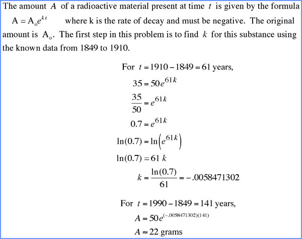
This section features . . . Radioactive Curves and CalculationsExample:
|
||
| days | hours |
years
|
||||||||||||||||||||||||||||||||||||||||||||||||||||||||||||||||||||||||||||||||||||
|
|
seconds
|
Half-lives of four common
radioisotopes: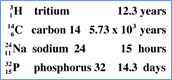 |
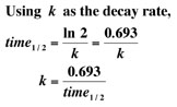
Experiment by entering data - the
decay rate k - from
above. Be sure to enter a
negative (-) in the rate representing exponential decay. |
Warning: Be
sure to enter half-lives with the same units of time - all years, days,
or hours. Otherwise comparisons in one graph are obviously not
valid. |
 |
Background:
|
Plot of carbon-14 decay rate against age
of the sample in years.
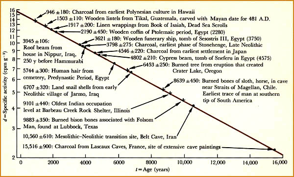 Historically known datable points (Ptolemaic period in Egypt) permited researchers to verify the concept of radiocarbon dating. |
Different radioisotopes have different half-lives. These range from fractions of a second to billions of years. However, with few exceptions, the only radioisotopes found in the natural world are those with long half-lives ranging from millions to billions of years. In 1947 the chemist Willard Frank Libby developed carbon-14 dating techniques leading to his Nobel Prize (1960). His methods are now found in a variety of situations. Carbon-14 has a half-life of 5,730 years, which may sound like a large number. But on the scale of existence of the universe, this half-life is quite small and thus a convenient yardstick for researchers. Carbon-14 dating is especially popular with anthropoligists seeking to date the age of bones. There are many other examples. Almost every biology lab will have a phosphate counter. Physicists have studied tritium decay seeking to understand fusion on the Sun. In the medical sciences, radioisotopes with short half-lives decay so rapidly that detection - imaging - is difficult. At the same time, the quality of rapid decay may be highly desirable for both diagnosis and therapy, e.g., chemotherapy. Clearly this is an important research topic. |
| From math class to
data in science and medical labs . . . Mathematics
texts usually treat both exponential growth (bacterial growth,
population growth, compound interest)
and exponential decay in the same chapter. All are logarithmic
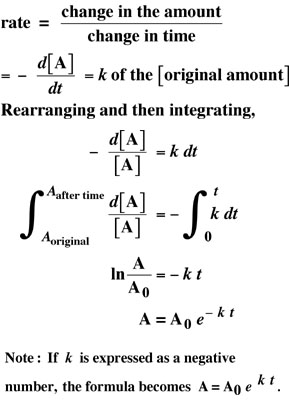
functions. But scientists
traditionally express rate constants as a positive number - though the
rate may represent an exponential decline. Thus we sometimes find
a difference between math texts and science texts in the formula for
decay. Science texts
will have a negative ( - ) in the exponent of the
formula for exponential decay.
|
 |
Useful
Links and Books |
 |
|||
| R. Chang, Physical Chemistry for the Biosciences, University Science Books, 2005, pp. 314-318. | |||||
|
R. E. Dickerson, H. B.
Gray, G. P.
Haight, Chemical Principles,
W. A. Benjamin, 1970, pp. 503-521.
|
|||||
| For a fascinating discussion of where radioisotopes are
being using in the medical sciences: < http://www.uic.com.au/nip26.htm >. |
|||||
| For decay as a
function of time: < http://www.lon-capa.org/~mmp/applist/decay/decay.htm >. |
|||||
| For more general
information on radioactive decay: < http://en.wikipedia.org/wiki/Radioactive_decay >. |
|||||
|
|||||