Back to . . . .
Tevian Dray
Oregon
State University
tevian@math.oregonstate.edu
NCB Deposit # 64
|

Vector Fields
|
JavaScript update
Jonathan Sahagun, 2018
jonathansahagun93@gmail.com
|
From the Vector Calculus Bridge Project -
Oregon State University
Vector
fields are vectors which change from
point to point. A standard example is the velocity of
moving air, in other words, wind. For instance, the current wind
pattern in the San Francisco area can be found at < http://sfports.wr.usgs.gov/cgi-bin/wind/windbin.cgi
>. This site has a 2-dimensional representation; careful
reading of the webpage will tell you at what elevation the wind is
shown. How would
you represent a vector field in 3 dimensions? What
features are important? Some simple examples are shown
below. Each can be rotated by clicking and dragging with the
mouse. Explore!
HOLD DOWN the mouse and
move it over
the vector field images on the left.
|
|
The first vector field
F1 on the left is constant. It
does not change from point to point. It therefore neither
diverges nor spins.
F1
= i
One question to ask
about a vector field is how it changes from point to point. Two
types of change are especially important: divergence and
curl. The divergence measures how much "stuff"
is "flowing" away from any given point; the
divergence is a function of position. The curl measures how
much "stuff" is rotating around a given point -- in a
given plane; the curl is itself a vector, and thus can contain
information about rotation in all planes.
But the key ideas are
"diverging" and "spinning".
|
|
|
F2 = x i + y j
The second vector field
F2 on the left is
clearly diverging from the center, but not spinning. Less obvious
is that it is also diverging from every other point.
If the wind were blowing like this, ANY two
nearby points would find themselves getting further and further
apart. For this reason, the radial vector field of
F2 can be thought of as "pure divergence".
|
|
|
F3 = -y i + x j
The
third vector field
F3 on the
left is clearly spinning about the center, but does not appear to
be diverging. Less obvious is that it also spins about every
other point.
A box placed in this current would not
only orbit about the center of the diagram, but also rotate about its
own center. This vector field represents "pure curl".
|
|
|
F4 = x i + y j + zk
Now compare
F2 with
F4 . The
former is in some sense 2-dimensional, since
F2 is the same in
every plane parallel to the xy-plane, whereas
F4 is
3-dimensional. Yet both appear similar in the original
2-dimensional representation.
|
|
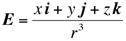
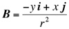
For the next two vector field images
be careful to distinguish the spherical
radial coordinate r
in E from
the cylindrical
radial coordinate r in B.
Physical fields tend to be more complicated than these first four
examples. For instance, the fifth vector field shown is the
Coulomb electric field E due to a point
charge at the origin, while the last is the magnetic field B
around an infinite wire along the z- axis carrying a steady
current. It may look as though these fields are again "pure
divergence" and "pure curl", respectively.
However, because these fields are weaker away from the center, some
things cancel. For instance, a small object would not rotate
about its center in wind which looked like B.
It turns out that E has divergence only at the
origin (where the divergence is infinite), and B
"spins" only along the z-
axis (where the curl turns out also to be infinite).
Maxwell's equations
for electromagnetism predict this behavior - the divergence
of the electric field tells you where the charges are, and the curl of
the magnetic field tells you where the currents are!
|
|
|
|
|
References
Please see Dr.
Dray's Bridge
Project.
< http://www.math.oregonstate.edu/bridge
>
< http://www.math.oregonstate.edu/bridge/ideas/fields
>.
|
| Further properties
of the divergence and curl -- in two dimensions
-- can be discovered using Matthias Kawski's vector field
analyzer found at < http://math.la.asu.edu/~kawski/vfa2
>. |
| Modern calculus texts will have extensive
material on vector calculus. James Stewart, Calculus, 5th
ed.,
THOMSONBrooks/Cole, 2003, Chapter 17, pp. 1090-1175. |
| Raymond Chang, Physical Chemistry
for the Biosciences,
University Science Books, 2005, pp. 25-26. |
| Donald A. McQuarrie, MATHEMATICAL
METHODS for Scientists and Engineers, University Science Books,
2003, (Section 7.1), pp. 191-197. |
Michael J. Crowe, A History of Vector Analysis: The
Evolution of the Idea of a Vectorial System, Dover, 1994.
|
Historical sketch . . .
The definitive history of vector analysis has been written by
Michael J. Crowe. In a nutshell, Hamilton
discovered quaternions, Maxwell found equations to describe
electromagnetism, and then Gibbs
and Heaviside rewrote Maxwell's theory in what is essentially the
modern language of vectors. The "i, j, k"
notation comes from Hamilton's quaternions.
|
|

James Clerk Maxwell
(1831-1879)
|

|
|
|

